8 One-way ANOVA
A one-way analysis of variance (ANOVA) is used when the independent variable is a nominal variable with more than two levels, and the dependent variable is continuous. There are two types of one-way ANOVA tests: a between-subjects ANOVA (just called ANOVA in jamovi) and a repeated measures ANOVA. The type of ANOVA you use will depend on whether your independent variable is between-subjects (standard ANOVA) or within-subjects (repeated measures ANOVA).
8.1 Independent One-Way ANOVA
Also called between-subjects one-way ANOVA, independent one-way ANOVAs are used when you have:
- 1 nominal independent/predictor variable
- The independent/predictor variable has more than 2 levels (conditions)
- Between-subjects design (participants complete only one level of the independent variable or are represented by one level of the predictor variable)
- A continuous dependent/outcome variable.
In this section, we will answer the research question, “Does well-being differ across the different regions of the U.S.?”.
8.1.1 Computing an Independent One-Way ANOVA
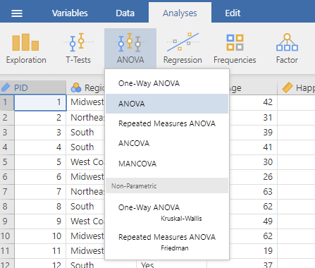
To compute an independent one-way one-way ANOVA, use the ANOVA menu: Analysis tab → ANOVA → ANOVA.
Note. There is a separate One-Way ANOVA option, but we want to use the ANOVA option instead. The ANOVA option will conduct the same test, and it allows you to request additional statistics, such as the effect size, which are required to report the test in APA style.
Add the continuous dependent variable you are interested in to the Dependent Variable window. Add the nominal independent variable to the Fixed Factors window. Under Effect Size, select ω2 (omega-squared).
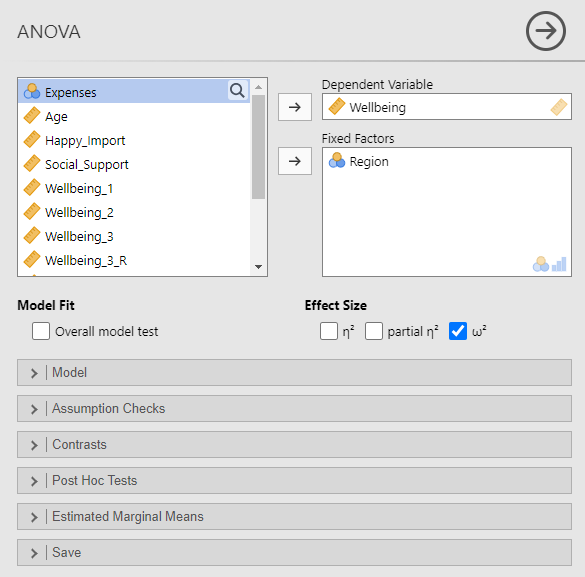
Note. It is not uncommon to see other effect size measures reported in psychology, such as η2 (eta-squared) and partial η2. However, these measures can be biased estimators, therefore the less biased ω2 is a better option for reporting effect sizes in ANOVA.[1]
These options produce the results tables below:
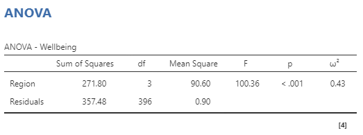
A significant one-way ANOVA tells us that at least two levels of the independent variable have significantly different levels of the dependent variable. However, it does not tell which levels are the same or different. To learn which levels are different from each other, we next need to conduct Post-Hoc Tests.
If the one-way ANOVA is not significant, there is no difference in the dependent variable across the levels of the independent variable. In other words, all groups have the same level of the dependent variable.
8.1.2 Follow Up a Significant Independent One-Way ANOVA
If your one-way ANOVA is significant, you will need to conduct post-hoc tests to determine which groups are different from which. In order to control for the error that results from conducting multiple tests, we’ll also want to use a statistical correction that adjusts our alpha level so that we don’t make a type 1 error (saying there is a significant difference when there is not). Jamovi has many options, but for a lot of complicated statistical reasons, we’re going to use the Holm correction (see section 13.5 of learning statistics with jamovi[2] if you want to learn about some of the complicated statistical reasons).
In the ANOVA menu, select the sub-menu Post Hoc Tests.
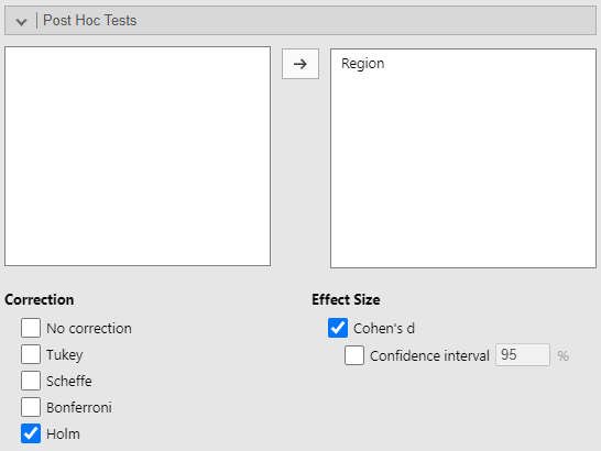
Move the independent variable to the right window. Under Correction, uncheck Tukey (the default) and select Holm. Under Effect Size, select Cohen’s d. These options will add a new table to your ANOVA results:
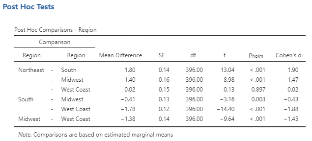
How to interpret the Post Hoc Comparison table:
- Line 1 indicates whether there was a significant difference in well-being for participants in the Northeast compared to the South.
- Line 2 indicates whether there was a significant difference in well-being for participants in the Northeast compared to the Midwest.
- Line 3 indicates whether there was a significant difference in well-being for participants in the Northeast compared to the West Coast.
- Line 4 indicates whether there was a significant difference in well-being for participants in the South compared to the Midwest.
- Etc.
8.1.3 Computing Means & Standard Deviations for an Independent One-Way ANOVA
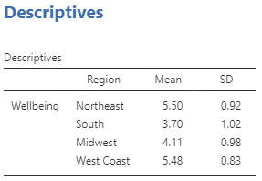
Just like in the t-tests, we will need to report the mean and standard deviation of the dependent variable for each level of our independent variable. Jamovi had a handy Descriptives option for t-tests, but a similar option for ANOVA does not include the standard deviations. We will have to calculate the means and standard deviation separately. See section 4.4 Descriptives by Group for how to do so.
8.1.4 Reporting an Independent One-way ANOVA
The results of a one-way between-subjects analysis of variance (ANOVA) indicated that participant well-being varied depending on what region of the U.S. they lived in, F(3, 396) = 100.36, p < .001, ω2= .43. Post-hoc tests (using the Holm correction) indicated that participants in the Northeast had higher well-being (M = 5.50, SD = 0.92) compared to those in the South (M = 3.70, SD = 1.02), t(396) = 13.04, pholm < .001, Cohen’s d = 1.90, and the Midwest (M = 4.11, SD = 0.98), t(396) = 8.98, pholm < .001, Cohen’s d = 1.47. There was no difference in well-being for participants in the Northeast compared to the West Coast (M = 5.48, SD = 0.83), t(396) = 0.13, pholm = .90, Cohen’s d = 0.02. Participants in the South had lower well-being compared to those in the Midwest, t(396) = −3.16, pholm = .003, Cohen’s d = −0.43, and those on the West Coast, t(396) = −14.40, pholm < .001, Cohen’s d = −1.88. Finally, participants in the Midwest had lower well-being compared to those on the West Coast, t(396) = −9.64, pholm < .001, Cohen’s d = −1.45.
Important Notes for Reporting Results
- Report the dependent variable mean and standard deviation for each group (level of the independent variable) in parentheses after you mention the group once (the first time the group is mentioned). We created the Descriptives table with these values in section 8.1.3.
- If the ANOVA was significant, then report the post-hoc tests. If the ANOVA is not significant, that means there was no difference in the dependent variable across the levels of the independent variable and no further tests are needed.
- For the F statement, in the parentheses put the degrees of freedom (df) from the ANOVA table line with the independent variable (in this case Region) first and the df from the line with the Residuals second.
- If a post-hoc test is significant, indicate which group was higher/lower on the dependent variable.
- Don’t forget the dependent variable and the comparison group! Participants in the Northeast have higher well-being compared to participants in the South. Make sure to describe the dependent variable and levels of the independent variable rather than using the variable name and level labels from jamovi.
- Make sure to include the effect size. For the ANOVA F-test, report ω2. For the post-hoc tests, report Cohen’s d.
- For notes on formatting statistical statements, see Appendix Reporting Statistics in APA style.
Another Option
When your predictor/independent variable has several levels, it is often more streamlined to report the means and standard deviations in an APA style table or figure rather than in text. When reporting results, report means and standard deviations either in-text or in a table/figure, but not both.
8.2 Repeated Measures One-Way ANOVA
Also called within-subjects ANOVA. Repeated measures ANOVAs are used when you have
- 1 nominal independent/predictor variable
- The independent/predictor variable has more than 2 levels (conditions)
- Within-subjects design (participants complete all levels of the independent/predictor variable)
- A continuous dependent/outcome variable.
A note on within-subjects designs and data organization
Recall that data is usually organized in jamovi so that every row represents a participant. Participants’ responses to each question in the well-being survey are then represented in each column. In between-subjects experimental research designs, it is common to have one column indicate what experimental condition the participant was in (this column is the independent variable) and additional columns for the participant’s responses to the dependent variable(s). In many of our examples so far each column represented just one variable (e.g., age, region, well-being, etc.). However, for within-subjects research questions, data is organized slightly differently. Because the research subject participates in all levels of the independent/predictor variable, there are multiple measures of the dependent/outcome variable, one for each independent/predictor variable level. For example, in addition to asking about generalized well-being, we also asked participants about their well-being in specific domains of their life: financial well-being, relationship well-being, and fun and recreation well-being. In our data, there is one column for each of these questions, but these three columns can represent multiple variables. If we are interested in the within-subject question “Does well-being differ across the three life domains?”, then the three columns represent both the predictor variable “life domain” and the outcome variable “well-being”.
In this section, we will answer the research question, “Does well-being differ across the three life domains?”.
8.2.1 Computing a Repeated Measures One-Way ANOVA
To compute a repeated measures one-way ANOVA, use the ANOVA menu: Analysis tab → ANOVA → Repeated Measures ANOVA.
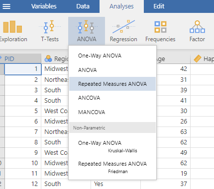
The Repeated Measures ANOVA menu looks a little different than the menus we have used so far:
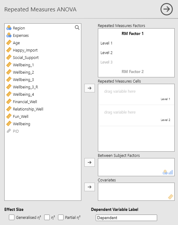
Because data is organized with rows representing participants and columns representing each question in our survey, the organization of variables is different for within-person variables. In this example, “Life Domain” is our independent variable with the levels: financial, relationship, and fun and recreation well-being. However, there is no “Life Domain” variable in our data set. Instead, we have three well-being variables that represent the three levels of Life Domain: financial well-being [Financial_Well], relationship well-being [Relationship_Well], and fun and recreation well-being [Fun_Well]. We need to tell jamovi that these three variables are actually different levels of one within-subjects independent variable.
In the Repeated Measured Factors window, select “RM Factor 1” and give it a meaningful name that represents your independent variable. The example below uses Life_Domain. Next, in the Repeated Measured Factors window, specify how many levels the variable has and give each level a name. When typing in the 3rd level (or higher), hit enter/return after you are done to add the level. The below example uses the level labels Financial, Relationship, and Fun. The level names you add will auto-populate to the levels in the Repeated Measures Cells window.
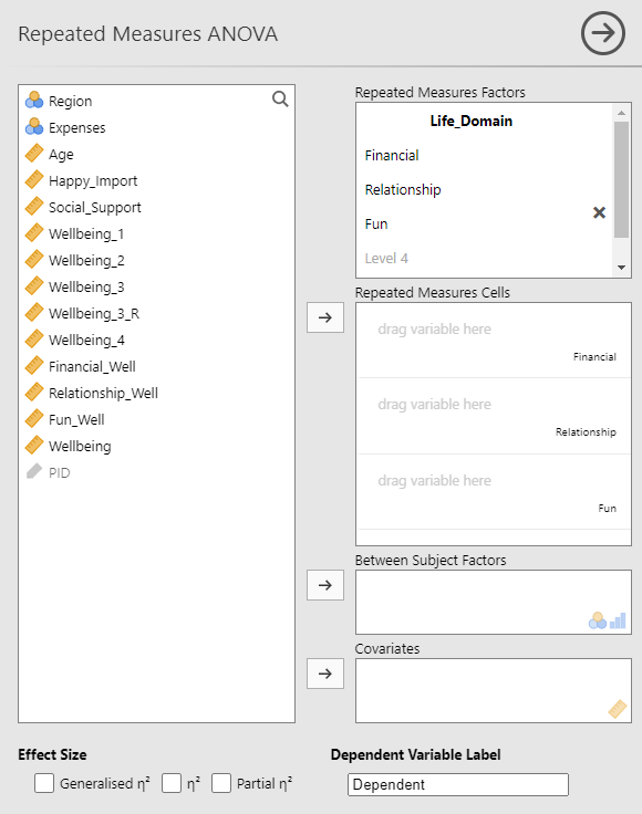
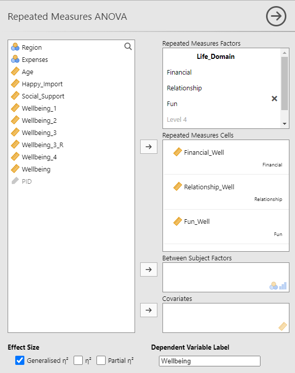
Next, add the variable from the list on the left that represents one of the levels of the independent variable to the corresponding cell on the right in the Repeated Measures Cells window. Give your dependent variable a name in the Dependent Variable Label window. The example below uses Wellbeing as the dependent variable name. Finally, under Effect Size, select Generalized η2.
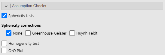
So far, we have not discussed the assumptions of the statistical tests we’ve covered and how to test if we have violated the assumptions. This is because the statistical tests we’ve covered to this point are pretty robust to violations of the assumptions (i.e., the assumption can be violated without serious error being introduced into the test). However, for repeated measures ANOVA we need to check if the assumption of sphericity is violated, and if it is violated, apply corrections to the F-value. To request the test of sphericity, use the Assumption Checks sub-menu and select Sphericity tests.
These options will add a new table to your repeated measures ANOVA results:

If the test is not significant (p > .05), then we have not violated the assumption of sphericity, and we do not need to apply any corrections to the F-value. If the test is significant (p < .05), then the assumption of sphericity is violated, and we need to apply a correction. If the Greenhouse-Geisser value is greater than .75 then use the Huynh-Feldt correction. If the Greenhouse-Geisser value is less than .75 then use the Greenhouse-Geisser correction. Both these options are available on the Assumption Checks sub-menu under Sphericity corrections. In this example, the test of sphericity is not significant, so we have not violated the assumption and do not need to apply a correction.
Now that we have checked the assumption of sphericity, we can turn to the results of the repeated measures ANOVA.
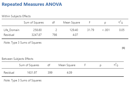
The first table is the within-subjects effects. A significant repeated measures one-way ANOVA tells us that at least two levels of the independent variable have significantly different levels of the dependent variable. However, it does not tell which levels are the same or different. To learn which levels are different from each other, we next need to conduct Post-Hoc Tests.
If the repeated measures one-way ANOVA is not significant, there is no difference in the dependent variable across the levels of the independent variable. In other words, all groups have the same level of the dependent variable.
The second table is the between-subjects effects. For this example, we did not include any between-subjects independent variables, so this table only lists residuals and has no significance test.
8.2.2 Follow Up a Significant Repeated Measures One-Way ANOVA
Just like the between-subjects ANOVA, if your one-way repeated measures ANOVA is significant, you will need to conduct post-hoc tests to determine which groups are different from which. In order to control for the error that results from conducting multiple tests, we’ll again want to use a statistical correction that adjusts our alpha level so that we don’t make a type 1 error (saying there is a significant difference when there is not). Jamovi has many options, we’re going to use the Holm correction.
In the Repeated Measures ANOVA menu, select the sub-menu Post Hoc Tests.
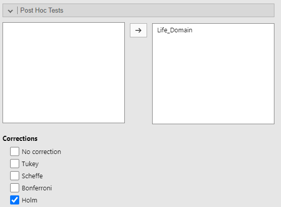
Move your independent variable to the right window. Under Corrections, unselect Tukey (the default) and select Holm. These options will add a new table to your ANOVA results:
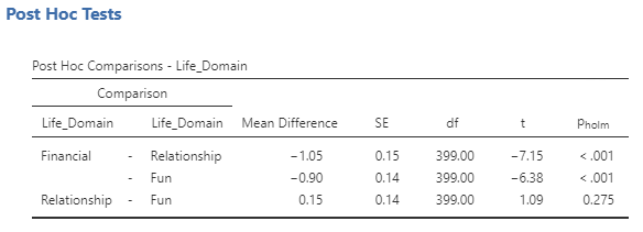
How to interpret the Post Hoc Comparison table:
- Line 1 indicates whether there was a significant difference between financial well-being and relationship well-being.
- Line 2 indicates whether there was a significant difference between financial well-being and fun and recreation well-being.
- Line 3 indicates whether there was a significant difference between relationship well-being and fun and recreation well-being.
8.2.3 Computing Means & Standard Deviations for Repeated Measures One-Way ANOVA
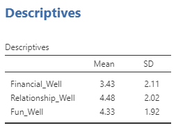
We will need to report the mean and standard deviation of the dependent variable for each level of our independent variable. Jamovi had a handy Descriptives option for t-tests, but a similar option for ANOVA does not include the standard deviations. We will have to calculate the means and standard deviation separately. Because we are dealing with a within-subjects measure, each level of the independent variable has its own variable in the dataset. So, we only need to request the descriptives for each of the variables that represent a level of our independent variable of interest. See section 4.3 Measure of Central Tendency, Variability, and More.
8.2.4 Reporting Repeated Measures One-Way ANOVA
The results of a one-way repeated measures analysis of variance (ANOVA) indicated that well-being differed across life domains, F(2, 798) = 31.79, p < .001, η2G = .05. Post-hoc tests (using the Holm correction) indicated that participants had lower well-being in the financial domain (M = 3.43, SD = 2.11) compare to their relationships well-being (M = 4.48, SD = 2.02), t(399) = −7.15, pholm < .001. Participants also had lower well-being in the financial domain compared to the fun and recreation domain (M = 4.33, SD = 1.92), t(399) = −6.38, pholm < .001. Finally, there was no difference between participants’ relationship well-being and their fun and recreation well-being t(399) = 1.09, pholm = .28.
Important Notes for Reporting Results
- Report the mean and standard deviation for each level of the independent variable in parentheses after you mention the level once (the first time the level is mentioned).
- If the repeated measures ANOVA was significant, then report the post-hoc tests. If the repeated measures ANOVA is not significant, that means there was no difference in the dependent variable across the levels of the independent variable, and no further tests are needed.
- For the F statement, in the parentheses put the degrees of freedom (df) from the Within Subjects Effects table line with the independent variable (in this case Life_Domain) first and the df from the line with the Residuals second.
- If a post-hoc test is significant, indicate which group was higher/lower on the dependent variable.
- Don’t forget the dependent variable and the comparison group! Participants had lower well-being in the financial domain compared to their relationship well-being. Make sure to describe the dependent variable and levels of the independent variable rather than using the variable name and level labels from jamovi.
- Make sure to include the effect size. For the repeated measures ANOVA F-test, report η2G (generalized eta-squared).
- For notes on formatting statistical statements, see Appendix Reporting Statistics in APA style.
Another Option
When your independent variable has several levels, it is often more streamlined to report the means and standard deviations in an APA style table or figure rather than report them in text. When reporting results, report means and standard deviations either in-text or in a table/figure, but not both.
