6 Multiple Regression
Multiple regression is used when you have more than one continuous predictor and a continuous outcome variable. Why not just calculate a series of correlations, like we did in the correlation chapter? When you calculate a set of correlations to look at the relationship between several predictor variables and an outcome variable, each individual correlation estimates the relationship between that predictor and the outcome variable but does not take into consideration the other possible predictor variable. Depending on your research question, this method may be appropriate! However, in psychology we are often interested in a predictor variable’s unique effect on the outcome variable. In other words, how much unique variance in the outcome variable is explained by the predictor variable, beyond the variance explained by other predictor variables. To answer this type of research question, we use multiple regression.
Multiple regression can also be used when you have both nominal predictor variables and continuous predictor variables, and a continuous outcome variable. Again, using multiple regression allows you to test each predictor variable’s unique effect on the outcome variable.
6.1 Computing Multiple Regression with Continuous Predictors
In this section, we will use age, how important happiness is to the participant, and social support as the predictor variables and well-being as the outcome variable (using our computed variable, the average of the four well-being items).
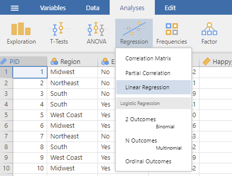
To compute a multiple regression, use the linear regression menu: Analysis tab → Regression → Linear Regression.
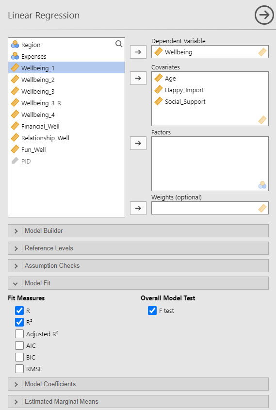
Add the continuous outcome variable you are interested in into the Dependent Variable window. Then add the continuous predictor variables to the Covariates window.
We will also want the statistical test of the overall model fit. To request this statistic, use the sub-menu Model Fit and select F test under Overall Model Test. The options for the Fit Measures R and R2 are selected by default.
These options produce the results tables below:
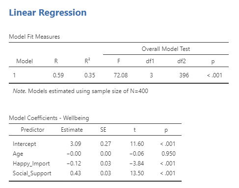
In multiple regression, the regression coefficients (in the Estimate column) now represent the unique, distinctive contribution of the predictor variable in explaining variance in the outcome variable, excluding any overlap with other predictor variables. The p-values in the Model Coefficients table indicate whether each predictor variable significantly predicts the outcome variable. By default, jamovi gives you the unstandardized regression coefficient (B) in the Estimate column. If you prefer standardized coefficients (β), you can request them in the Model Coefficients sub-menu under Standardized Estimate.
The R2 and the ANOVA significance test of the R2 now answer the question: Does the model (all of the predictors together) explain a significant amount of the variance in the outcome variable? In this example, age and happiness importance and social support (together) explain 35% of the variance in well-being. The Overall Model Test indicates that this is a significance amount of the variance in well-being.
6.2 Reporting Multiple Regression with Continuous Predictors in APA Style
We conducted a multiple regression analysis with age, happiness importance, and social support predicting subjective well-being. The model explained a significant amount of the variance in subjective well-being, R2 = .35, F(3, 396) = 72.08, p < .001. Participants’ age did not significantly predict their well-being, B = −0.00, SE = 0.00, p = .95. The more participants thought happiness was important for a meaningful life, the lower well-being they reported, B = −0.12, SE = 0.03, p < .001. Greater perceived social support was associated with higher levels of well-being B = 0.43, SE = 0.03, p < .001.
Important Notes for Reporting Results
- The first sentence should describe the model. Next, report if the model explained a significant amount of the variance in the outcome variable.
- Use descriptions of the variables rather than the variable names from jamovi. E.g., “participants thought happiness was important for a meaningful life” rather than “Happy_Import”.
- When a predictor is significant, always interpret the direction of the relationship rather than just saying it is significant. As one variable goes up, what happens to the second variable? For example, as X variable increased, Y variable decreased (a negative relationship), or higher levels of X variable were associated with greater levels of Y variable (a positive relationship).
- B denotes an unstandardized regression coefficient and is found in the Estimate column.
- If you report B and SE, you do not need to report the t-statistic (because t = B ÷ SE and, therefore, is redundant information).
- If you choose to report standardized regression coefficients, only report β and the p-value.
- For notes on formatting statistical statements, see Appendix Reporting Statistics in APA Style.
6.3 Computing Multiple Regression with Nominal and Continuous Predictors
Sometimes you have both nominal predictor variables and continuous predictor variables that you want to use to predict a continuous outcome variable. Multiple regression can do that too!
In this section, we will use how important happiness is to the participant, social support, and whether participants have enough money to cover their monthly expenses (a two-level nominal variable) as the predictor variables and well-being as the outcome variable (using our computed variable, the average of the four well-being items).
To compute a multiple regression, use the linear regression menu: Analysis tab → Regression → Linear Regression.

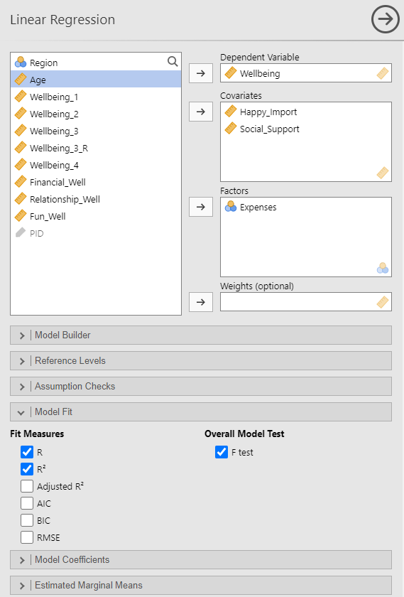
Add the outcome variable you are interested in into the Dependent Variable window. Add the continuous predictor variables to the Covariates window. Add the nominal predictor variable to the Factors window.
We will also want the statistical test of the overall model fit. To request this statistic, use the sub-menu Model Fit and select F test under Overall Model Test. The options for the Fit Measures R and R2 are selected by default.
Tip
In the bottom right of each of the variable windows on the right half of the Linear Regression menu is a symbol that indicates what variable type is appropriate for that window. In the Dependent Variable window, we see the ![]() continuous variable symbol because in linear regression dependent/outcome variables must be continuous. In the Covariates window, we also see the
continuous variable symbol because in linear regression dependent/outcome variables must be continuous. In the Covariates window, we also see the ![]() symbol, which indicates that continuous predictors belong in this window. And in the Factors window, we see the
symbol, which indicates that continuous predictors belong in this window. And in the Factors window, we see the ![]() nominal variable symbol, indicating that nominal predictors belong in this window.
nominal variable symbol, indicating that nominal predictors belong in this window.
These options produce the results tables below:
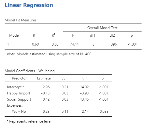
Just like before, p-values in the Model Coefficients table tell you whether each predictor variable significantly predicts the outcome variable. In this analysis, the nominal predictor variable Expenses (whether participants have enough money to cover their monthly expenses) was significant. Below the variable name are the two levels of the variable, Yes – No. Looking at the regression coefficient (in the Estimates column), we see that the coefficient is positive. This means the first level listed had higher levels of the outcome variable compared to the second level listed (also called the reference level). In other words, participants who reported having enough money to cover their monthly expenses (the “Yes” group) had higher well-being compared to those who did not have enough money to cover their monthly expenses (the “No” group). If the nominal predictor is significant and the regression coefficient is negative, that means the first level listed had lower levels of the outcome variable compared to the second level listed. Finally, if the nominal predictor is not significant, then there was no difference in the outcome variable between the two levels of the predictor variable.
6.4 Reporting Multiple Regression with Continuous and Nominal Predictors in APA Style
We conducted a multiple regression analysis with happiness importance, social support, and whether participants have enough money to cover their monthly expenses predicting subjective well-being. The model explained a significant amount of the variance in subjective well-being, R2 = .36, F(3, 396) = 74.44, p < .001. The more participants thought happiness was important for a meaningful life, the lower well-being they reported, B = −0.13, SE = 0.03, p < .001. Greater perceived social support was associated with higher levels of well-being B = 0.42, SE = 0.03, p < .001. Whether participants had enough money to cover their monthly expenses significantly predicted well-being such that those who could cover their monthly expenses had higher well-being compared to those who could not, B = 0.23, SE = 0.11, p = .03.
Important Notes for Reporting Results
- The first sentence should describe the model. Next, report if the model explained a significant amount of the variance in the outcome variable.
- Use descriptions of the variables rather than the variable names from jamovi. E.g., “participants thought happiness was important for a meaningful life” rather than “Happy_Import”.
- When a continuous predictor is significant, always interpret the direction of the relationship rather than just saying it is significant. As one variable goes up, what happens to the second variable? For example, as X variable increased, Y variable decreased (a negative relationship), or higher levels of X variable were associated with greater levels of Y variable (a positive relationship).
- When a nominal predictor is significant, report which level of the variable had higher (or lower) levels of the outcome variable compared to the second level of the variable (also called the reference level).
- B denotes an unstandardized regression coefficient and is found in the Estimate column.
- For notes on formatting statistical statements, see Appendix Reporting Statistics in APA Style.
